How to build a Neural Network in Python to compute XNOR¶

By Joel Pendleton

Introduction¶

This is a tutorial using Python on how to create a basic neural network to generate a function to perform the XNOR operation.

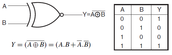
An XNOR gate (sometimes referred to by its extended name, Exclusive NOR gate) is a digital logic gate with two or more inputs and one output that performs logical equality. The output of an XNOR gate is true when all of its inputs are true or when all of its inputs are false. If some of its inputs are true and others are false, then the output of the XNOR gate is false.

Mathematics and Algorithms¶

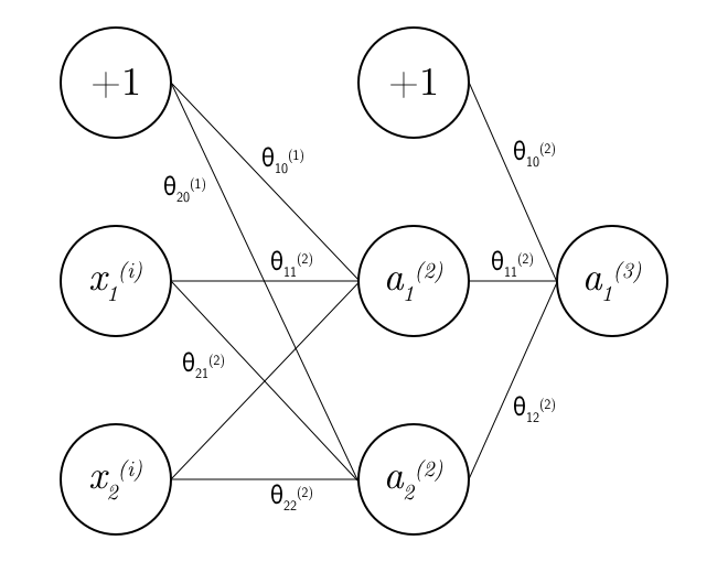
This is the architecture of the neural network used in this tutorial:

The activation function used in this network is the sigmoid function: $$ g(x) = \frac{\mathrm{1} }{\mathrm{1} + e^{-x} } $$

The derivative of the sigmoid function, $ g^{'}(x) $ can be to shown to be $$ g^{'}(x) = g(x)(1 - g(x)) $$

If you're wondering why you would want to use the sigmoid function, I'd recommend taking a look at these resources:

The cost function used is $$J(\theta) = \frac 1m \sum_{i=1}^m\sum_{k=1}^k\begin{bmatrix}-y_k^{(i)}\log((h_\theta(x^{(i)}))_k) - (1-y_k^{(i)})\log(1-(h_\theta(x^{(i)}))_k)\end{bmatrix} + \frac{\lambda}{2m} \sum_{l=1}^{L-1}\sum_{i=1}^{s_l}\sum_{j=1}^{s_l + 1}(\theta^{(l)}_{ij})^2$$
The cost function tells you how well your model fits the provided data. The smaller the cost the better your model. Therefore, we want to minimise the cost. We do this by varying our parameters in a manner that reduces the cost. This is accomplished by the back propagation algorithm.

The second term is a regularization term. I never used regularization so $\lambda = 0$ and you can effectively ignore this term.
$k$ is the number of output units in scenairo $k = 1$ as there's only 1 output unit.
$l$ is the layer number, e.g. for a unit on layer 1, $l = 1$.
$s_l$ is the number of units, excluding bias units on layer $l$.
$i$ specifies the unit of a layer.
$j$ specifies the weights of a unit.

import matplotlib.pyplot as plt
import numpy as np

def sigmoid(z):
    return 1 / (1 + np.exp(-z))


def sigmoid_derivative(z):
    return sigmoid(z) * (1 - sigmoid(z))

#These functions are used in the later code.

x = np.arange(-10., 10., 0.2)
plt.plot(x,sigmoid(x), '-k', label="Sigmoid")
plt.legend(loc='upper left')
plt.xlabel("z")
plt.ylabel("g(z)")
plt.show()

Forward Propagation Algorithm¶

Algorithm for our 3 layer neural network:

$a^{(1)} = x$
$z^{(2)} = \theta^{1}a^{(1)}$
$a^{(2)} = g(z^{(2)})$ (add $ a^{(2)}_{0}$)
$z^{(3)} = \theta^{2}a^{(2)}$
$a^{(3)} = g(z^{(3)})$ (Output) $$ a^{(1)} \in \mathbb{R}^{3} $$ $$ a^{(2)} \in \mathbb{R}^{3} $$ $$ a^{(3)} \in \mathbb{R}^{1} $$

Forward propagation is used to find what our model predicts for each training example. This will tell us how we should tune our weights ($\theta$) to make our model more accurate. This tuning of weights is done using backpropagation.

Back Propagation Algorithm¶

Import training set {$(x^{(1)},y^{(1)}), ..., (x^{(m)},y^{(m)})$}
set $\Delta^{(l)}_{ij} = 0$
For $i = 1$ to $m$
- Perform forward propagation to compute $a^{(1)}, a^{(2)}, ... a^{(L)}$
- Using $y^{(i)}$ compute $\delta^{(L)} = a^{(L)} - y^{(i)}$
- Compute $\delta^{(L-1)}, \delta^{(L-2)}, ..., \delta^{(L)}$
  - $\delta^{(L)}= a^{(1)}_{j} - y_{j}$
  - $\delta^{(n)}= (\theta^{(n)})^{T}\delta^{(n - 1)} \odot g^{'}(z^{(n)}) $, where $n < L$
- $\Delta^{(l)}_{ij} := \Delta^{(l)}_{ij} + a^{l}_{j}\delta^{(l + 1)} $
- $D^{(l)}_{ij} := \frac{1}{m}\Delta^{(l)}_{ij} + \lambda\theta^{(l)}_{ij}$ if $ j \neq 0$
- $D^{(l)}_{ij} := \frac{1}{m}\Delta^{(l)}_{ij}$ if $ j = 0$

You can think of $\delta^{(n)}$ as the error in our model at layer n.
$ \lambda$ is the regularization parameter. In our code example $\lambda = 0$

Using our cost function, we can write: $$ \frac{\partial}{\partial\theta^{(l)}_{ij}} J(\theta) = D^{(l)}_{ij}$$
Therefore, $ D^{(l)}_{ij}$ can be used in an optimisation algorithm to minimise the cost function. In our code, we have done this using the gradient descent algorithm. For more on gradient descent, I'd recommend reading https://ml-cheatsheet.readthedocs.io/en/latest/gradient_descent.html

This algorithm above is the general algorithm, we will make it specific to our case by setting $L = 3$, $m = 4$, and $n = 1, 2$.

$$ \theta^{(1)}, \Delta^{(1)}, D^{(1)} \in \mathbb{R}^{2 x 3} $$$$ \theta^{(2)}, \Delta^{(2)}, D^{(2)} \in \mathbb{R}^{1 x 3} $$

N.B. $\theta^{(1)}$ and $\theta^{(2)}$ are weights of layer 1 and layer 2, respectively.

Putting it all together¶

Initialise weights
Implement forward propagation to get
Implement backpropagation to compute partial derivatives
for i = 1 to m
- Perform forward and back propagation using training example $(x^{(1)},y^{(1)})$
Use gradient descent or another optimisation method with backpropagation to minimise $J(\theta)$ as a function of parameters / weights $\theta$.

The cost function $J(\theta)$ is non-convex so you may get a different minimum value and 'optimised' parameters based on what you initialise $\theta$ as.

Python Code¶

Create Training Data¶

Here I have made an array of possible values of $x_1$ and $x_2$ and their corresponding outputs and put them into numpy arrays.

X = np.array([[0,0],
             [0,1],
             [1,0],
             [1,1]])

y = np.array([[1],
      [0],
      [0],
      [1]])

Neural Network Object¶

Using Python's OOP features I have created a Neural Network class.

class NeuralNetwork:

    def __init__(self, X, y):
        self.X = np.c_[np.ones((X.shape[0], 1)), X] #Training inputs
        self.y = y # Training outputs
        self.numberOfExamples = y.shape[0]  # Number of training examples
        self.w_1 = (np.random.rand(2, 3) - 1) / 2  # Initialise weight matrix for layer 1
        self.w_2 = (np.random.rand(1, 3) - 1) / 2  # Initialise weight matrix for layer 2

        # Error in each layer
        self.sigma2 = np.zeros((2,1))
        self.sigma3 = np.zeros((3,1))

        self.predictions = np.zeros((4,1))

        # There is 2 input units in layer 1 and 2, and 1 output unit, excluding bias units.

    def feedforward(self, x):

        self.a_1 = x  # vector training example (layer 1 input)
        self.z_2 = self.w_1 @ self.a_1
        self.a_2 = sigmoid(self.z_2)
        self.a_2 = np.vstack(([1], self.a_2))  # Add bias unit to a_2 for next layer computation
        self.z_3 = self.w_2 @ self.a_2
        self.a_3 = sigmoid(self.z_3) # Output
        return self.a_3

    def backprop(self):

        # These are temporary variables used to compute self.D_1 and self.D_2

        self.d_1 =  np.zeros(self.w_1.shape) 
        self.d_2 = np.zeros(self.w_2.shape)
        
        # These layers store the derivate of the cost with respect to the weights in each layer
        self.D_1 = np.zeros(self.w_1.shape)
        self.D_2 = np.zeros(self.w_2.shape)

        for i in range(0,self.numberOfExamples):

            self.feedforward(np.reshape(self.X[i, :], ((-1,1))))
            self.predictions[i,0] = self.a_3
            self.sigma3 = self.a_3 - y[i] #Calculate 'error' in layer 3
            self.sigma2 = (self.w_2.T @ self.sigma3) * np.vstack(([0],sigmoid_derivative(self.z_2))) #Calculate 'error' in layer 2
            '''We want the error for only 2 units, not for the bias unit. 
            However, in order to use the vectorised implementation we need the sigmoid derivative to be a 3 dimensional vector, so I added 0 as an element to the derivative.
            This has no effect on the element-wise multiplication.'''
            self.sigma2 = np.delete(self.sigma2, 0)  # Remove error associated to +1 bias unit as it has no error / output
            self.sigma2 = np.reshape(self.sigma2, (-1, 1))

            # Adjust the temporary variables used to compute gradient of J
            self.d_2 += self.sigma3 @ (self.a_2.T)
            self.d_1 += self.sigma2 @ (self.a_1.T)

        # Partial derivatives of cost function
        self.D_2 = (1/self.numberOfExamples) * self.d_2
        self.D_1 = (1/self.numberOfExamples) * self.d_1

    def probs(self, X): #Function to generate the probabilites based on matrix of inputs
        
        probabilities = np.zeros((X.shape[0], 1))
        for i in range(0, X.shape[0]):
            test = np.reshape(X[i,:], (-1,1))
            test = np.vstack(([1], test))
            probabilities[i, 0] = self.feedforward(test)
        return probabilities

Create Neural Network Object and Perform Gradient Descent¶

# Neural network object
nn = NeuralNetwork(X,y)


alpha = 1  # Learning Rate

for i in range(0, 2000): #Perform gradient descent
    nn.backprop()

    # Update weights
    nn.w_1 += - alpha * nn.D_1
    nn.w_2 += - alpha * nn.D_2

Contour Map¶

The code below is just the plot of the contours of the output. Although the inputs in this case are discrete variables, I thought it would be interesting to visualise the decision boundary.

xx, yy = np.mgrid[-0.1:1.1:0.1, -0.1:1.1:0.1]

grid = np.c_[xx.ravel(), yy.ravel()]

# Find the probabilities for each combination of features

probs = nn.probs(grid).reshape(xx.shape)

f, ax = plt.subplots(figsize=(12, 10))

# Create contour lines for each set of probabilities

contour = ax.contourf(xx, yy, probs, 25, cmap="RdBu", vmin=0, vmax=1)

plt.title("x$_1$ XNOR x$_2$")
ax_c = f.colorbar(contour)
ax_c.set_label("$P(y = 1 | X)$")
ax_c.set_ticks([0, .25, .5, .75, 1])

# Plot training examples on figure

ax.scatter(X[:,0], X[:, 1], c=y[:,0], s=50,
           cmap="RdBu", vmin=-.2, vmax=1.2,
           edgecolor="white", linewidth=1)

ax.set(aspect="equal",
       xlabel="x$_1$", ylabel="x$_2$")


plt.show()

This notebook was created in an attempt to consolidate what I've learned from Andrew Ng's Machine Learning course: https://www.coursera.org/learn/machine-learning

Moreover, I'd highly recommend the following resources for learning more about neural networks:

Thanks for reading :)